Thevenin
FUEL_GAUGE_THEVENIN estimates the SOC with an extended Kalman filter over a
Thevenin equivalent circuit: the cell’s \(R_0\) in series with one RC
polarization pair. Coulomb counting predicts the SOC, and the measured
terminal voltage corrects it, so the estimate doesn’t drift with current
errors nor jump with the load.
Model
The cell is an equivalent circuit: the OCV of the cell, in series with its resistor \(R_0\) and one resistor-capacitor pair \(R_1 \parallel C_1\).
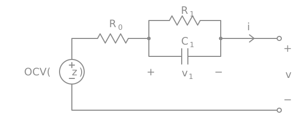
Thevenin equivalent circuit of the cell, with the current \(i\) positive when discharging.
With \(z\) the SOC (0 to 1), \(i\) the current (positive when discharging), \(Q\) the capacity in coulombs and \(v_1\) the voltage across the RC pair, the terminal voltage \(v\) follows
\(R_1 \parallel C_1\) is the slower polarization (charge transfer and diffusion). It builds up under load and relaxes with the time constant \(\tau_1\) once the load is removed. Without the pair (\(R_1 = 0\)), the model is \(R_0\) alone.
A single RC pair keeps the model small and its fit well conditioned. Dynamics much faster than the sample interval can’t be resolved anyway, so more pairs only pay off with faster sampling.
Discretization
Samples come at times \(t_k\), with \(\Delta t_k = t_k - t_{k-1}\). The current \(i_k\) is a single sample taken at \(t_k\), and it is held over the whole interval \((t_{k-1}, t_k]\). For a constant current, the RC equation has the exact solution
and coulomb counting gives
The estimator and the fit use these same equations, so a model fitted on bench logs behaves the same way in the firmware, whatever the sample interval.
Temperature
Resistances grow as the cell gets colder. Both \(R_0\) and \(R_1\) are scaled by
with \(T\) in °C, clamped to -20..60 °C, and \(\kappa\) the resistance temperature coefficient. The OCV and the capacity don’t depend on temperature.
Filter
The estimator is an extended Kalman filter over the state \(x = [z, v_1]^T\) and its covariance \(P\). Each measurement \((v_k, i_k, T_k)\) goes through a prediction and a correction.
Predict (coulomb counting), with \(g_k\) the sensitivity of the state to the current:
The process noise comes only from the current error \(\sigma_i\)
(current_noise). Both states are driven by the same current, so its
covariance is the outer product of \(g_k\) with itself. \(\sigma_i\) is how far
the single sample \(i_k\) can be from the true average current of the
interval. With sparse samples and a bursty load, this dominates over the
error of the current measurement itself.
Correct (voltage). The predicted terminal voltage and its linearization:
\(e_k\) is how far the measured voltage is from the predicted one, and \(S_k\)
its expected variance. \(\sigma_v\) (voltage_noise) covers the voltage
measurement error and the model error.
How much the correction moves the SOC depends on the OCV slope \(\mathrm{OCV}'\), but the gain on \(z\) isn’t proportional to it. Ignoring \(v_1\), the gain is \(K_z = P_{zz}\,\mathrm{OCV}' / (\mathrm{OCV}'^2 P_{zz} + \sigma_v^2)\): it first rises with the slope, then falls as \(1/\mathrm{OCV}'\) where the curve is steep, since there a voltage error is a small SOC error. What rises with the slope is \(H K\), the fraction of the voltage error \(e_k\) the correction removes. With \(\sqrt{P_{zz}} = 2\%\) and \(\sigma_v = 15\) mV, on the OCV curve of a small Li-po cell charged to 4.45 V:
Where |
\(\mathrm{OCV}'\) (V) |
\(K_z\) (1/V) |
\(H K\) |
|---|---|---|---|
plateau, 7.5-10% |
0.43 |
0.58 |
0.25 |
near full, 95-100% |
1.1 |
0.62 |
0.68 |
near empty, 0-1% |
26.6 |
0.038 |
1.00 |
So on the flat plateau the filter mostly keeps the coulomb count, and where the curve is steep it follows the voltage almost entirely. Current gain and offset errors, which make pure coulomb counting drift without bound, are corrected continuously.
Charge complete. When the charger terminates, the SOC is set to 1 with a small uncertainty.
Parameters
struct pbl_fuel_gauge_estimator holds them. In the firmware they come from
Kconfig, through PBL_FUEL_GAUGE_ESTIMATOR_KCONFIG:
Parameter |
Kconfig |
|---|---|
\(R_1\) |
|
\(\tau_1\) |
|
\(\kappa\) |
|
\(\sigma_v\) |
|
\(\sigma_i\) |
|
Characterization below describes how \(R_1\), \(\tau_1\) and \(\kappa\) are measured and fitted, together with the cell.
Limitations
The OCV is modelled at 25 °C, and the capacity doesn’t depend on temperature. Only the resistances do.
\(R_0\) and \(R_1\) don’t depend on the SOC, while those of a real cell rise near empty. Close to empty, the model then underestimates the drop under load.
There is no OCV hysteresis between charge and discharge. The fitted curve sits between the two branches when the logs include charging.
Capacity fade with aging is not tracked.
Characterization
This section describes how to measure a cell and fit this model to it: what to measure, with which instrument, and how to check the result. Models come only from our own measurements. The method doesn’t depend on an instrument; Characterization tools has the tools that implement it.
The flow is:
Charge the cell as the product does, rest it, and discharge it in pulses down to the cutoff, logging voltage, current and temperature.
Fit the model to the log with
tools/fuel_gauge/fuel_gauge.py fit, which writes a model file and prints the board’s battery node properties and Kconfig defaults.Check it, with
fuel_gauge.py replayon the bench log, then on a second cell or on logs from the device.
Full and empty
The model’s SOC runs from 0 to 1 between two points that the procedure defines, so they have to be the product’s.
Full (\(z = 1\)) is where the charger terminates. Charge with the product’s charge profile: the same termination voltage, charge current and termination current as the device (the battery node in the board’s devicetree). A different profile moves “full” and changes the capacity.
Empty (\(z = 0\)) is where the discharge stops: the cutoff voltage, under the load of the last pulses. The estimator reports 0% at \(z = 0\), and the battery service treats 0% while unplugged as critical, so the cutoff defines where the device reports empty. Choosing it is a product decision: a lower cutoff gives more runtime, a higher one leaves more margin before the cell’s protection or the PMIC’s brownout.
The capacity \(Q\) is the charge delivered between these two points, at the procedure’s discharge rates.
Instrument
The procedure needs a programmable load and a charger (or a way to swap between them), and logs of the following, with the reasons:
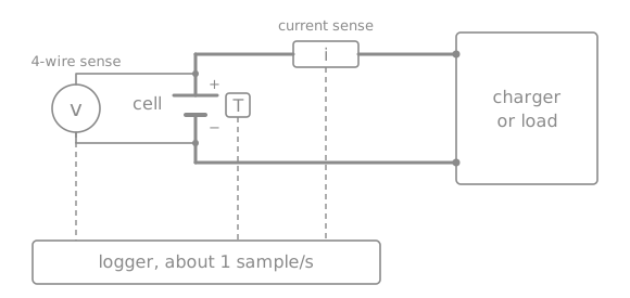
sense at its terminals and a temperature sensor, all read by a logger
Measurement setup. The force path runs through the current sense to the charger or load, while the voltage is sensed separately at the cell terminals. Voltage, current and temperature are logged together.
Voltage at the cell. Everything between the cell and the voltage sense point ends up in \(R_0\). Use 4-wire sensing at the cell terminals, or measure the fixture’s resistance \(R_\text{fixture}\) between the cell and the sense point. The device measures at its own PMIC, through its own path \(R_\text{device path}\), so the model’s resistance is
\[ R_{0,\text{model}} = R_{0,\text{fit}} - R_\text{fixture} + R_\text{device path}.\]Resolution of a few millivolts is enough: the fit residual of a good model is 5-10 mV.
Current, with a known error. The fit takes the SOC from coulomb counting, so a current error becomes a capacity error, and through it an error on the SOC of every OCV point. With a gain error \(\epsilon_i\) and an offset \(i_\text{off}\) over a test of length \(T\):
\[ \frac{\delta Q}{Q} \approx \epsilon_i + \frac{i_\text{off}\, T}{Q}.\]The offset counts over the whole test, rests included, which are most of it. For a 70 mAh cell over a 15 h test, a 1% capacity error allows only about 47 µA of offset. Check the instrument’s specification against this budget, and check the current logged during the rests, which should read 0.
Sample rate of about 1 Hz. The fit sees \(R_0\) in the voltage step at each pulse edge and \(\tau_1\) in the relaxation after it, which takes tens of seconds; the samples have to resolve both.
Temperature of the cell, or at least of the ambient, since the resistances depend on it. Characterize at a stable temperature, away from heat sources.
Test profile
A constant-current discharge can’t separate the OCV from the resistive drops: at a constant \(i\), \(R_0 i\) and \(R_1 i\) are just offsets on the OCV. Pulses with rests make every parameter visible:
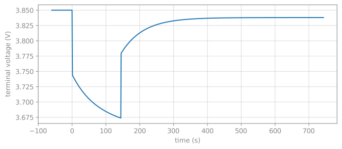
The step at each pulse edge is \(R_0\, s(T)\, \Delta i\).
The relaxation after a pulse of current \(i\) and length \(t_p\) is
\[ R_1\, s(T)\, i\, \left(1 - e^{-t_p/\tau_1}\right) e^{-t/\tau_1},\]which gives \(R_1\) and \(\tau_1\). The RC pair only charges to \(1 - e^{-t_p/\tau_1}\) of \(R_1 s(T) i\) during the pulse: 89% for a 144 s pulse at \(\tau_1 = 65\) s, 51% at \(\tau_1 = 200\) s.
The end of each rest is close to the OCV at that SOC, as long as the relaxation has died out.
The profile’s parameters, and what sets them:
Parameter |
Default |
Why |
|---|---|---|
Initial rest |
30 min |
The log has to start from a full cell at rest: right after charging, the polarization of the CV phase is still relaxing. |
Pulse depth |
2% of \(Q\) |
Each pulse gives one OCV point, so 2% gives about 50, at least two per interval of a 21-25 point OCV grid. Shallower pulses lengthen the test. |
Pulse rate |
0.5C |
The step \(R_0 \Delta i\) has to stand well above the voltage resolution (about 100 mV for a 70 mAh cell with a 3 Ω \(R_0\)), without heating the cell. |
Pulse length |
depth / rate, 144 s |
At least about \(\tau_1\), so the RC pair charges enough for its relaxation to show. |
Rest |
until relaxed |
See below. |
Tail |
quarter rate, 4× long |
Near the cutoff, from 0.2 V above it under load: a lighter load draws more charge before the cutoff, closer to the device’s. |
Rest criterion. A rest should end once the remaining relaxation is below the error the OCV points can tolerate. For an exponential, the voltage still to relax is \(\tau_1\, |dv/dt|\), so with \(\tau_1\) up to 200 s, leaving less than 1 mV takes \(|dv/dt| < 5\) µV/s, about 0.3 mV/min. Measure the slope over a few minutes, as it is below the voltage resolution over a single second. An instrument that can’t end a step on a condition needs a fixed rest long enough for the slowest expected \(\tau_1\): 15 minutes is 4.5 to 9 time constants for \(\tau_1\) of 100 to 200 s, and about 14 for 65 s.
The discharge takes about 15 hours, plus the charge.
Fit
python tools/fuel_gauge/fuel_gauge.py fit mycell_25c.csv --name mycell -o mycell.json \
    --grid 0 0.01 0.02 0.03 0.05 0.08 0.1 0.15 0.2 0.25 0.3 0.35 0.4 0.45 \
    0.5 0.55 0.6 0.65 0.7 0.75 0.8 0.85 0.9 0.95 1
The capacity, \(R_0\) and the OCV curve go in the board’s simple-battery
node (charge-full-design-microamp-hours,
factory-internal-resistance-micro-ohms and ocv-capacity-table-0). The RC
pair and the temperature coefficient go in the board’s Kconfig.defconfig,
as defaults of FUEL_GAUGE_THEVENIN_RC_MILLIOHM,
FUEL_GAUGE_THEVENIN_RC_TAU_MS and FUEL_GAUGE_THEVENIN_R_TEMP_COEFF_PPM
under if FUEL_GAUGE_THEVENIN, so they only apply where the model is used.
The devicetree takes the OCV curve in whole percents, so the grid points
must be whole percents too.
By default each log starts full (--start-soc 1), and the first log ends
empty (--end-soc 0), which defines the capacity. --capacity-ah sets it
instead. The fit prints the parameters, the voltage residual, and a warning
for any SOC range the logs don’t cover. fit --help has the options.
To fit the temperature coefficient, run the procedure at other temperatures
too (e.g. 5 °C and 40 °C, in a climate chamber) and pass all logs to fit.
The first log defines the capacity, so put the 25 °C one first.
Known SOC path
The fit needs the SOC at every sample, which coulomb counting provides when the log starts from a known state:
A log that starts full (\(z_0 = 1\)) and ends at the cutoff (\(z_\text{end} = 0\)) defines the capacity:
Linear least squares
For a fixed \(\tau_1\) and \(\kappa\), the terminal voltage is linear in all the other unknowns. Writing the OCV as linear interpolation over a grid of SOC points \(z_1 < \dots < z_n\),
where \(w_j\) are hat functions (each sample has at most two non-zero weights), the model becomes
with \(\ell\) the first-order lag of the discretization, \(\ell_k = a_k \ell_{k-1} + (1 - a_k)\, s(T_k)\, i_k\). Stacking all \(N\) samples gives an overdetermined linear system \(A\theta \approx v\) in \(\theta = [\mathrm{OCV}_1 \dots \mathrm{OCV}_n, R_0, R_1]\).
Three constraints make the solution physical:
Increasing OCV. The OCV points are written as a base voltage plus steps, \(\mathrm{OCV}_j = u_1 + \sum_{m=2}^{j} u_m\), i.e. \(\mathrm{OCV} = T u\) with \(T\) a lower-triangular matrix of ones, and every step \(u_m \ge 0.1\) mV. The estimator requires a strictly increasing curve, and a non-increasing one would make the SOC ambiguous.
Non-negative resistances, \(R_0, R_1 \ge 0\).
Smoothness. A penalty \(\lambda \lVert D_2 T u \rVert^2\) on the second difference of the OCV fills SOC ranges without data and damps noise, with \(\lambda = \text{smoothing}^2 N / n\) (
--smoothing). The data term grows with \(N\), so scaling \(\lambda\) with it keeps the penalty’s effect independent of the log length.
Nonlinear parameters
\(\tau_1\) and \(\kappa\) enter nonlinearly. For each candidate, the linear problem is solved and its residual kept (variable projection), so the outer search only explores one or two dimensions:
\(\tau_1\): bounded 1-D minimization of the mean squared residual over \(\ln \tau_1 \in [\ln 5, \ln 5000]\) s.
\(\kappa\): when the logs span at least 10 °C, a bounded 1-D minimization over \([0, 0.08]\) 1/°C, each candidate with its best \(\tau_1\). Otherwise it is fixed at 0.03 1/°C, a typical value for Li-ion cells.
Grid
The default grid is 21 evenly spaced points (--grid-points, or --grid
for explicit points). The OCV bends sharply near empty, so a grid denser
there, like above, fits the end of the discharge noticeably better. Grid
points that no sample falls next to are reported, since their OCV comes only
from the smoothness penalty.
Validate
Residual. Around 5-10 mV RMS is a good fit. Large maximum residuals tend to sit at the very end of the discharge, where the OCV bends sharply; a denser grid there helps.
Coverage warnings. An SOC range without data means the procedure didn’t reach it, typically near full (charge not completing) or near empty (cutoff too high).
Parameters. \(R_0\) and \(R_1\) of a few hundred milliohms up to a few ohms are normal for small cells, \(\tau_1\) of tens to a few hundred seconds.
Replay.
replay --start-soc 1runs the firmware estimator over the log and compares it against coulomb counting:python tools/fuel_gauge/fuel_gauge.py replay mycell.json mycell_25c.csv --start-soc 1 --plot soc.png
This checks the model and the estimator together, but on the data the model was fitted to. A second cell of the same type, or logs from the device, is a stronger check.
synth simulates the bench procedure on an existing model, quarter-rate
tail included, which shows how well a profile identifies the parameters
without running it:
python tools/fuel_gauge/fuel_gauge.py synth mycell.json synth.csv --lsb 0.0049
python tools/fuel_gauge/fuel_gauge.py fit synth.csv --name test -o fit.json
On simulated device usage (one sample a minute of a 1 mA load with 20 mA bursts, 5 mV voltage resolution), a model that matches the cell keeps the SOC within about 1%. That still holds with a ±10% current gain error or a ±0.3 mA offset. A start 20% off converges within minutes. On a real cell, the model error dominates, so the fit residual is the number to watch.
Limitations of the method
Resistances from discharge pulses. \(R_0\) and \(R_1\) are fitted on 0.5C discharge pulses, and the model uses them for charging at up to 1C too. Charge and discharge resistances differ, and so may the resistance at other rates, and the fixture resistance adds to the fitted \(R_0\) unless it is measured. The model’s \(R_0\) is the one to check on device charge logs.
Constant resistances. \(R_0\) and \(R_1\) are fitted as one value over the whole SOC range, while a real cell’s rise near empty, so the fit there trades resistance error for OCV error.
One temperature. Without logs at several temperatures, \(\kappa\) is the default 0.03 1/°C.
No hysteresis. The procedure only discharges. The OCV after charging sits slightly higher than after discharging; the model has a single curve.
Rate-dependent capacity. The capacity is what the profile draws down to the cutoff. A lighter load gets a little more out of the cell; the low-current tail reduces the difference.
Aging. One fresh cell is measured, and capacity fade isn’t modelled.